Basically : Aquaculture Production Simulation
The Zoo-technical base is a : Thermal Profile, (mean weekly temperature), a general Daily Growth Model, and a Daily Feeding Table.
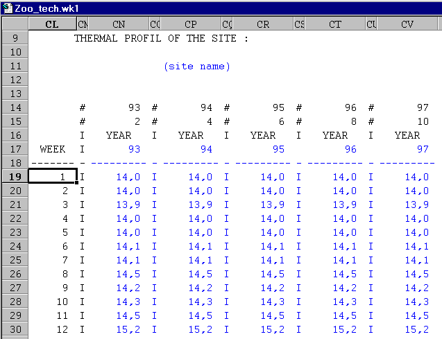
An example of a thermal profile is : etc….
This table contains the mean fish weight (row), the temperature (column) and the manufacture’s, or anyone’s, suggested daily percentage (intersection) of food based upon the number of individuals. This calculates into Kilos of food to distribute which can provide cost per kilo calculations and other “bottom line” considerations.
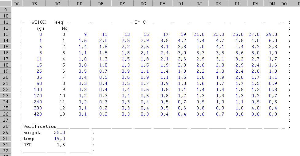
Weight – (column DB in this example) is in grams.
Seq. No – is a necessary internal values and must not be modified!
T° – C – is the water temperature in Celsius.
Daily Feeding Rate – is at the intersection of Weight and T°-C
Verification – is a user work area to test the results of the table. Enter the weight and temperature. The DFR found in the table is displayed, in this case 1,5. Note : the column “seq.” is used to locate the row number in the horizontal look-up.
|
DAILY FEEDING TABLE – DFT SEABASS DAILY FEEDING TABLE (from IFREMER) Weight 1 to 420 g – Temp 9° to 29°C
|
The model shown below is a : general growth model for Sea Bass (D. labrax) weighing between 1 and 500 grams and a temperature between 14.5 and 26 °C.
The Daily Growth Model, is obtained from Leclercq & Tanguy, which calculates the weekly weight gain.
By changing the values of the Daily Growth Rate (DGR) it is possible to simulate other species growth function.
|
The formula and factors used to calculate the DGR are : DGR =aWd-0.34 x e0.12t W = Weight of the fish in grams
If the temperature is less than 14.5° or greater than 26oC (Formula from LECLERCQ & TANGUY, 1988) |
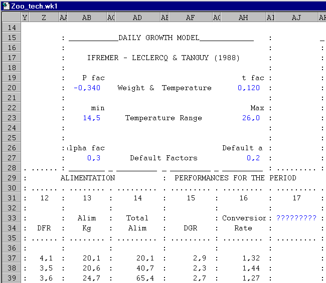
The daily growth model is represented as series of variables shown below. Changing the values in blue will effect the growth calculations for the animals. Thus this model can be adapted to other species..
Zoo-Tech Introduction
eZoo-Tech is an introductory spread sheets applications applied to marine aquaculture production. It provides important, easy to understand calculations with user controlled information.
There are three sections in Zoo-Technical, Control, Tabls and Calculations.
Zoo-Technical
The simulation is based upon a site’s Thermal Profile, (mean weekly temperature), a general Daily Growth Model, and a Daily Feeding Table plus other information and models.
Control
The user can vary simulation (production) parameters which are grouped into 7 categories :
- Period – Beginning, ending date
- Stock – Number, mean weight, individual price
- Mortality – Percentage and number
- Daily Growth Model – Ranges, factors, default values
- Environment – Consumption of O2, production NH3 + NH4, …
- Cage – Size, length,
- Food Characteristics – Granulo, price,
Calculations
In this example calculations are intermixed with their controls. This is done in order to better demonstrate “cause and effect” and hyerartical control. In SIM and SAP controls are centralized and seperated from calculations.
|
Note 1 : Everything in color,
|
|
Note 2: Screen shots are provided to indicate the coordinates of the area in question |
Control Section
Period – Beginning, ending date
The beginning date and ending date of the simulation. Note there must be enough rows to complete all the calculations. One row per week. Each row calculate its results based upon the previous week’s results.
Time step is the number of days the Growth Rate model requires to perform it’s calculations.
No. Weeks is the number of weeks between the beginning date and ending date.
Stock – Number, mean weight, individual price
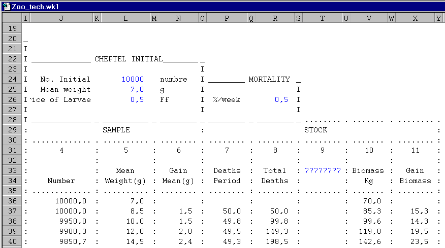
The user indicate the initial number of individuals, their mean weight (in grams) and the mean price of an individual.
Mortality – Percentage and number
A constant percentage of individual which will die each week.
Daily Growth Model – Ranges, factors, default values
The user can modify the constants which control the growth model. Thus the model can be adapted to other species or refined for a specific site.
For further details see Daily Growth Model.
Environment
Environment information concerns particulate matter, nitrogen and other metabolic products. Plus O2 consumption, the required minimum percent of hourly water exchange, the weekly and total production of ammoniac, etc.
Several formulas are provided to estimate production of waste products.
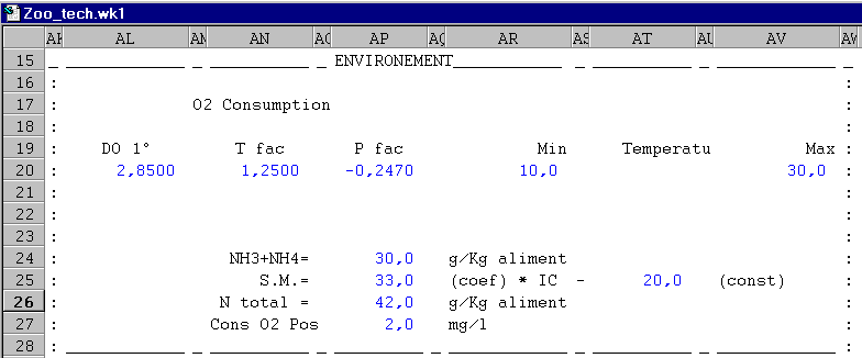
Nitrate Production (NH3+NH4 = 30.0 g/Kg Food) – ammonium and organic nitrogen production rate, is in grams – ie. 30 and 42 respectively – produced per Kg of food.
Total Nitrogen (N total = 42.0 g/Kg Food) – production is calculated as grams per Kilogram of food provided.
Particulate Matter Production (33.0 (coef)*IC-(const) 20.0 ) – coefficient – i.e. 33,0 – times the conversion rate minus a constant – i.e. 20,0.
Concentration of O2 Possible (Cons. O2 possible 2.0 mg/l) – the normal amount of dissolved oxygen (O2), mg per litter of sea water.
Nitrate & Nitrogen Production
Food to Nitrate Production, ammonium and organic nitrogen production rate, in grams is calculated using the amount of food provided – i.e. 30 grams and 42 grams respectively, produced per Kg of food given to the fish.
Total nitrate & nitrogen production is calculated as grams per Kilogram of food provided. Default values are :
NH3+NH4 = 30.0 g/Kg Food
N total = 42.0 g/Kg Food
Suspended Particle Production
The conversion of food to particulate matter (P.M.) is a coefficient, calculated using a constant (i.e. 33,0) multiplied by the conversion rate minus a constant, i.e. 20,0.
P.M. = (33.0 *CR) – 20.0
Oxygen Consumption
A O2 consumption model works on the same principle as the Daily Growth Model, that is an initial mean weight and weekly temperature.
Daily O2 Consumption = 2.8500 constant 1.2500 (T fac) -0.2470 P facThe factors of this calculation are :
Daily O2 Consumption Rate is a mean hourly rate in mg per liter.
An initial value of 2mg of O2 per liter present the normal amount of dissolved oxygen (O2), in mg per litter of sea water.a Temperature range from a minimum of 10.0 °C to a maximum of 30.0 °C
General O2 Consumption Model valid for Seabass from 1 to 700 g Temperatures range from 10 to 30°C
(IFREMER/Palavas, 1989)
Cage – Characteristics of the cage
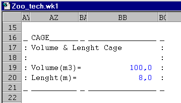
Cage Volume (m3) & Cage Length (m) is required in order to calculate current speeds and water recycling within the cage. The length of the cage is in relation to the water current.
Food Characteristics - Granulo, price
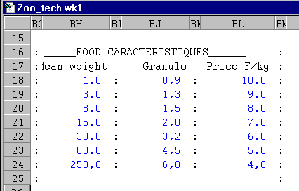
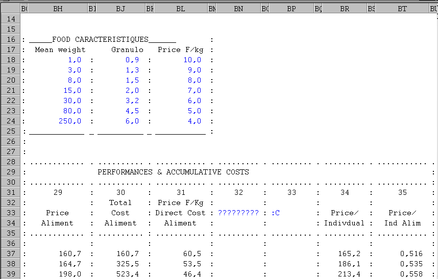
The user establishes a food characteristic table indicating a food size, or granulo, for a mean weight and its cost per kilo. As the simulation advances and the animals gain weight the corresponding granulo and price are correctly selected thus effecting food costs, animal value, etc.
Mean Weight – the average size (weight in grams) of the fish and the size of the food particles (or granulo) they eat.
Granulo – the different sizes (usually in diameter) of foods available as feed.
Price (units / kilo) – cost of the feed in units (in this case French Francs) per kilo.
|
Note : You are free to place any mean weight, granulo and cost combination required. This includes other foods (grains, inscects,etc.) You must respect an ascending sequence in the weigth column. The simulation retains the first weight which doesn’t exceed the size of the fish. |
Calculations Section
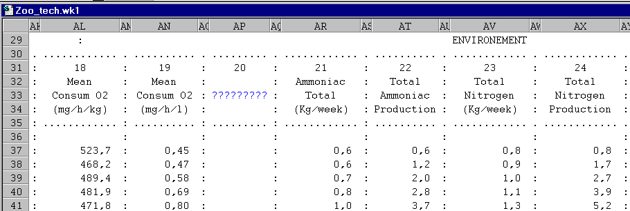
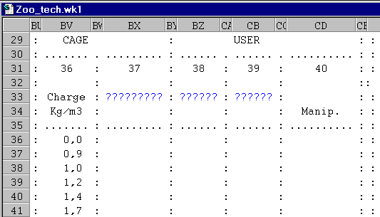
Results are displayed in columns (column numbers are in parenthesis, grouped by theme :
Period,Sample,
Alimentation,
Performance & costs
Environment
Cage
The calculations performed in this area (i.e. the mean temperature, number of individuals, mean weight, mortality and total mortality), are dependent upon the initial data entered in the area PERIOD, STOCK and MORTALITY
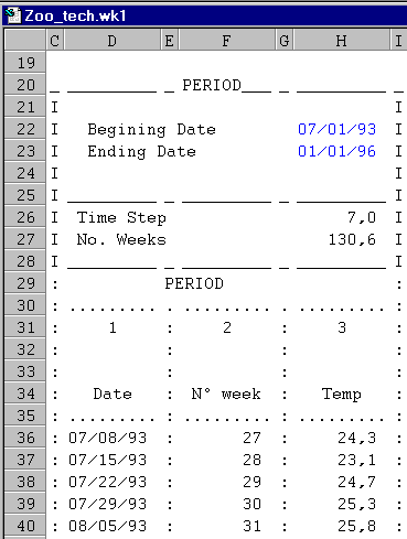
Date (1) – The date contains the initial or previous date plus the time step.
Week number (2) – The date is converted to the week number.
Temp (3) – The temperature is obtained from the site’s Thermal Profile. This two-dimensional “look-up” table is access via the year and the week number, both are
obtained from the date.
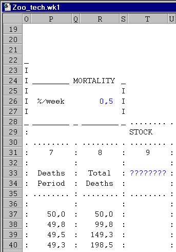
Number (4) – The number is the result of the initial or previous number minus the weekly moralities.
Mean Weight (g) (5) – The mean weight is calculated using the Growth Rate Model, initial or previous weight and the mean weekly temperature.
Gain Mean (g) (6) – The gain in mean weight is the difference from one week to the next.
Deaths Period (7) – Mortality is the result of multiplying the percentage of mortality per week by the number.
Total Deaths (8) – Cumulating deaths for the period provides a “running total” of all deaths.
User’s Choice (9) – Any additional calcualtion can be entered into this column.
Biomass Kg (10) – The product of the mean individual weight and the number of individuals.
Gain Biomass (11) – The difference in biomass from one period to another.
Alimentation present the results of feeding ratio, daily growth and conversion rates.
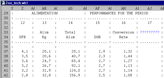
Daily Feeding Rate (DFR) (12) – The value present here is obtained using a two-dimension look-up of the Daily Feeding Table. The DFR is the percentage of food required for a given biomass which is a function of the temperature and mean weight of the animal.
Alimentation Kg (13) – The alimentation provided is the product of the DFR and the biomass.
Total Alimentation (14) – The running total of alimentation provided.
Daily Growth Rate (DGR) (15) – This value is obtained using the Daily Growth
Model, Thermal Profile, and the individual weight of the organism.
Conversion Rate (also know as Conversion Index) (16) – The result of dividing the total aliments by the biomass.
User’s Choice (17) – Any additional calcualtion can be entered into this column.
Mean and maximum O2 consumption in mg/h/kg and mg/h/l

Mean weekly Consumption of O2 (18 & 19) – Using the O2 consumption model, the mean weight and temperature the consumption is calculated in mg per hour per Kg and mg per hour per litter.
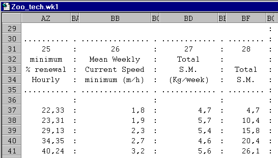
Ammonica and Total Ammoniac (21 & 22) – The amount of ammoniac produced is the product of the Kg of food provided and the NH3 + NH4 factor established above. The total ammoniac is a running total of all ammoniac
produced.Total Weekly Nitrogen and Total Nitrogen Produced (23 & 24) – Like ammoniac, nitrogen production is the product of the Kg of alimentation distributed and the N coefficient described above. Total nitrogen produced is a running total of all N produced.
Minimum % Renewal Hourly (25) – This calculation is based upon the length of the cage in relation to the predominate current, the biomass and the maximum concentration of O2 in solution.
Mean Weekly Current Speed (minimum in meters/hour) (26) – This value is calculated using the cage length and the percent of renewal per hour required to flush the cage with oxygenated water.
Total Particulate Matter (P.M.) & Total P.M. (27 & 28) – This metabolic by-product is calculated as the product of P.M. coefficient (described above) and the conversion index minus a constant i.e. 20.
The resulting calculations are indicative – the results are provided for discussion purposes.
This section presents data concerning food costs.
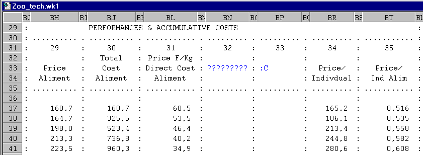
Price of Aliment (29) – The weekly cost of food based upon the total aliment (14) and the food characteristic table.
Total Cost of Aliment (30) – This is the running total of alimentation costs.
Price (in cost per Kg) Direct Cost of Alimentation (31) – This is the cost of producing a Kilogram of fish, in food cost only.
Price per Individual (34) – The value initial plus the value of the food distributed per individual.
Price per Individual in Alimentation (35) – The value of an individual in the cost of food it has consumed.
Calculates the biomass and density with the cage.
Charge Kg/M3 (36) – The density or biomass per cubic meter.
Last updated 02/06/10 06:43:28
