
SIM REAL
Sim_Real combines real production data with simulated results. It is based upon ZOO_TECH, but provides further insight into spread sheet uses and their potential.
By combining : REAL weekly production data, (i.e. number of fish moved (in/out), mortality, mean weight and kilos of food distributed) with user controlled initial data (i.e. starting date, number initial, etc.) the user can quickly summarize production for short-term results based upon real and current trends.
In many simulations, each week’s calculated results are based upon the previous weeks result’s. This can cause the simulated results to “drift” each week from the actual production data. After several months the simulated results could vary greatly from real production data.
The main advantage of updating simulation data with real production data is to re-calibrate the simulation and understand the causes of the drift.
|
Note 1 : Everything in color, i.e. blue or green, (this depends upon how your program i.e. Excel, Lotus, VisiCalc, etc., is configured), is what you can change to adapt the spread sheet to your examples. |
|
Note 2: Screen shots are provided to indicate the coordinates of the area in question |
Real Vs. Simulated Data
As in ZOO_TECH, the user establishes initial conditions (Start date, Number of Fish, Mean Weight, Price per larvae, Mean percentage of mortality per week). In addition the user can select between 2 different growth models (i.e. IFREMER and user defined).
Once the weekly calculations are performed the user can enter data such as :
Real Number Exchanged – actual number of fish removed or added to the cage
Real Mean Weight(g) – actual measured mean weight (in grams) of the fish.
Real Mortality – number of fish which actually died.
Real Food (Kg) – amount of food distributed to the fish.
If this data is entered into correct week – or row, the simulation will take into consideration the new information and calibrate the simulation accordingly.
For example : if the Real Number Exchanged is modified (it is usually left blank) by adding fish, or by subtracting fish ( a negative value) then the simulated number of fish will change which will then effect all other calculations (i.e. bio-mass, feeding, costs, etc.).
The Real Mean Weight(g) is a value obtained by actually measuring selected individuals (or the whole lot) and averaging their weight. This, when entered into the simulation will effect all subsequent calculations concerning bio-mass, feeding, etc.
Real Mortality is the actual number of dead fish found each week. As fish grow their death rate changes causing serious problems for simulations based upon fix death rates. By entering the actual number dead the simulation avoids the fixed death rate while providing precious information concerning the actual size, age and cost of dead fish.
Real Food (Kg) is the amount of food distributed during the week. Feeding tables provided by feed suppliers are based many considerations. The actual amount of food distributed re-calibrates everything associated with food (i.e. costs, conversion and growth rates, etc.) plus providing insight into the actual functioning of the aquaculture site (local growth models, feeding table, etc.)
By logging basic weekly production data the simulation has access to important information which when compared “side-by-side” indicate how to fine tune the simulation and actual production.
Simulation Control
In Sim_Real control of the simulation is centralize in one location, the Control Section while more static information is stored in the zoo-technical section. In ZOO_TECH, controls are placed over the columns they effect.
Starting Date – this is the beginning date which is transformed into a week number and year. This determines the temperature returned from the Thermal Profile, which in turn effects growth and all other the calculation performed. It is important that the Starting Date be contained in theThermal Profile time period.
Number of fish – beginning number of individuals.
Mean Weight – the weight (mean) of an individuals.
Price per Larvae – the cost of an individual fish. The currency in not required and assumed that the same currency is used to purchase foods and evaluate costs.
% Mortality per Week – a fixed rate which remains constant throughout the simulation.
Cage Volume – the volume of the cage is necessary in order to calculate the density.
Growth Model Selection Switch is a flag which controls which Daily Growth Model to use when calculating growth and consumption values. As described in ZOO_TECH the Daily Growth Model is a “general” model and not specific to anyone production method or farm. Thus a second model is provided which allows the user to set their own parameters for growth.
% Mortality real – During the simulation real data is entered, such as the number of dead fish each week. The real number of dead fish is converted to percentage and posted to this field.
Time step for DGR (in days) – The Daily Growth Model is based upon one week ( 7 days). The model and means are calculated using this value. It is possible to configure for another time step (i.e. 14 days, 30 days, etc.).
The effects of modifying the time step can be unpredictable.
User’s Daily Growth Model
This is the general Daily Growth Model as presented in Sim_Real. It is the same as found in ZOO_TECH.
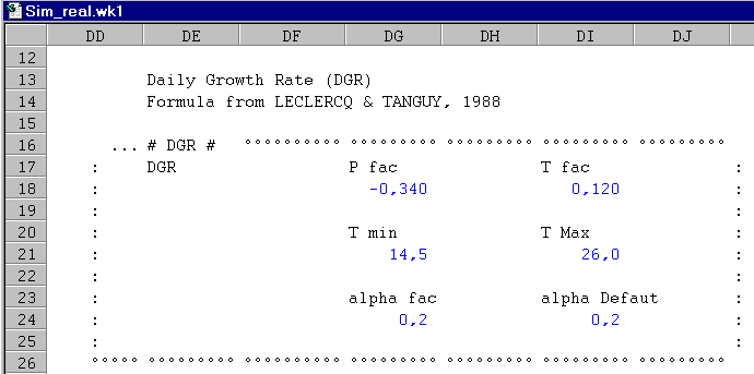
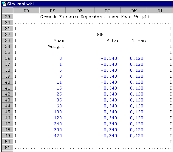
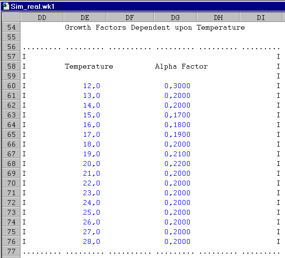
This is a user developed growth model. It “breaks out” the general Daily Growth Model into smaller weight, growth and temperature steps. By modifying the P and T factors for a give mean weight the user can approach the same growth rates as observed at their production sites.
Several points need to be clarified.
1) the P factor influences the growth rate more than the T factor.
2) the mean weight values and its associated P and T factors should remained grouped as to effect a size range as opposed to individual weight.
3) technically it is possible to reverse engineer a growth model if enough “real “information is provided (this feature has yet to be implemented).

As described above the weight (P factor) can easily off-set minor differences associated with the temperature. I recommend that the user modify the P factor and verify the calculation before modifying the P factor.
Characteristics of the Alimentation
Alimentation is now presented in a two dimensional table with the granule (row), the purchase date (column). Their intersection contains the price paid per kilo of food. Seven different types of “granule” can be defined and purchased at 12 different dates.
The user “estimates” the date and price per kilo (without taxes) and the computer will calculate the cost, based upon the mean weight of fish, the date and the daily feeding table.
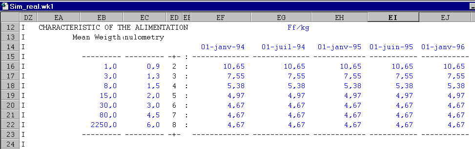
Mean Weight – the average size (weight in grams) of the fish and the size of the food particles (or granulo) they eat.
Granulo – the different sizes (usually in diameter) of foods available as feed.
Date and Purchase Price (units / kilo) – cost of the feed in units (in this case French Francs) per kilo purchased on a specific date. This price per kilo is employed to calculate all feed cost for the simulation until the next date and purchase price combination.
|
Note : You are free to place any mean weight, granulo and cost combination required. This includes other foods (grains, insects,etc.) |
Performance
Performance as measured economically in food and individual costs.
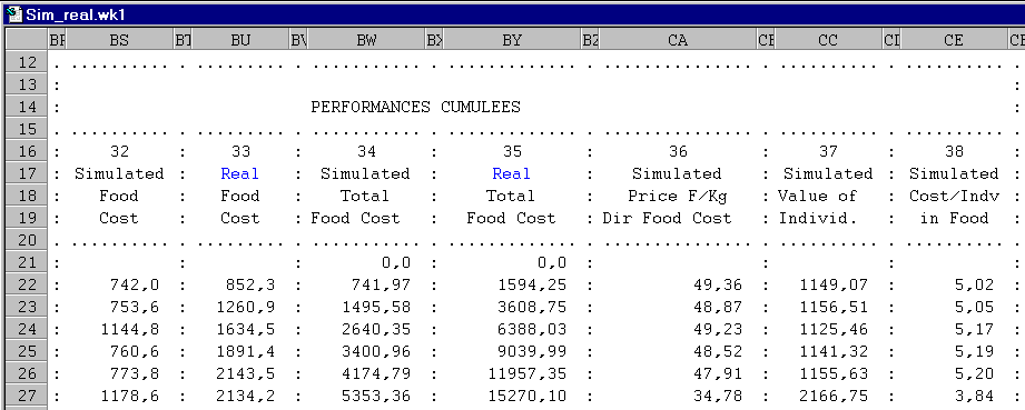
Simulated Food Cost (32) – the results of a look up of the Characteristics of the Alimentationusing the Simulated Mean Weight (g) (6) to obtain the granulo and the Real & Simulated Date (1) to obtain the Purchase Price (units / kilo). The Purchase Price (units / kilo) is multiplied by the Simulated Food kg (21).
Real Food Cost (33) – the multiplication of the Real Food Kg (22) distributed and Price (units / kilo).
Simulated Total Food Cost (34) – the running total of the Simulated Food Cost (32).
Real Total Food Cost (35) – the running total of the Real Food Cost (33).
Simulated Price (units/kilo) Direct Food Cost (36) – this is the original cost of the lot (Number of fish multiplied by the Price per Larvae plus the Simulated Total Food Cost (34) divided by the Simulated Biomass (Kg) (16). This give the value (in costs per kilo produced) of the cheptel, but only based upon purchase price and food costs.
Simulated Value of Individual (37) – Real & Simulated Number (4) divided by the Simulated Price (units/kilo) Direct Food Cost (36). The value added to an individual in food costs alone.
Simulated Cost per Individual in Food (38) – this is the sum of the Simulated Price (units/kilo) Direct Food Cost (36) and the Simulated Biomass (Kg) (16) divided by the Real & Simulated Number (4). The cost of every individual just in food.
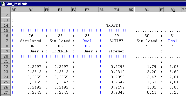
Growth
This section pertains to the growth models used to simulate production. As is the case with all models, their predictive abilities are base upon many factors which often vary in non-controlled environments,. such as production. This section was designed to adapt a growth model to a specific situation, a single cage. The problem is complicated due to a lack of accurate information and sampling methods. However this does not mean that the problem is unsolvable.
Simulated DGR – Users (26) – shows the results the user’s growth model obtained.
Simulated DGR – IFREMER (27) – shows the results the general growth model obtained.
Real DGR User’s (28) – currently not used. This column was reserved to calculate the real daily growth rate based upon sampled (real) data.
Active Growth Model (29) – is selected using the Growth Model Selection Switch, which is in the Control section. In this case the switch is set to “0” which set the Simulated DGR – IFREMER (27) will be used as the basis for following calculations
Simulated Conversion Index (30) – this is the Simulated Food kg (21) divided by the Gain Biomass (Kg) (18) which provides us with the rate food is converted to biomass.
Real Conversion Index (31) – is the Real Food Kg (22) distributed divided by theGain Biomass (Kg) (18).
Period
A column’s value could be a combination of real and simulated data. For example 1) Real & Simulated Date which starts with real data which is entered by the user. The simulation then calculates all subsequent weeks. 2) Week No is a pure calculation based only upon the dates 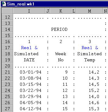 provided in the 1) Real & Simulated Date column.
Columns with both blue (or green) and black text indicates that real data is used to initialize the column but all other data is calculated.
Real & Simulated Date (1) – the first date is real, as it is obtained from the control section. But, all the others dates are simulated.
Week No (2) – the result of converting the date to a week number.
Real & Simulated Temperature (3) – the results of a lookup of the Thermal Profile using the year from the Real & Simulated Date (1) and the Week No (2). The temperature is both real but obtained from simulated data, the Real & Simulated Date (1).

This sections shows columns with text in both blue and black and other columns all in blue. As stated above blue and black text indicates real data which is entered by the you and used to 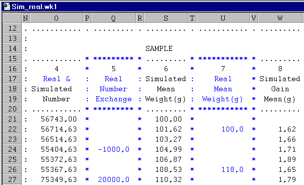 initiate or adjust calculations. All blue text indicates a column which requires “real” user data.
Real & Simulated Number (4) – This column is effected by the Starting Number, Real Number Exchanged and Real Mortality.
The Starting Number of individuals decreases based upon the % Mortality per Week. However, should the user enter a value in the Real Number Exchange (5) (for example adding or removing individuals) this value will re-adjust Real & Simulated Number (4). The simulation will continue based upon this new information.
In the example below 1000 fish are removed (-1000). This will effect many different columns such as biomass, kilos of alimentation, etc.
Real Number Exchange (5) – The number of individual exchanged. A negative value indicates the removal of individuals.
Simulated Mean Weight (g) (6) – This column is completely simulated and based upon the Daily Growth Model.
Real Mean Weight (g) (7) – As in Real Number Exchange (5), this column stores the mean weight, as measured by sampling individual.
Simulated Gain Mean Weight (g) (8) – This column is completely simulated and based upon the weekly differences in Simulated Mean Weight (g) (6).

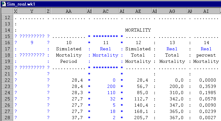 This series groups and describes the mortality associated with production
User’s Choice (9)– Any additional calculation can be entered into this column.
Simulate Mortality Period (10) – This is calculated based upon the value established in the control % Mortality per Week.
Real Mortality (11) – The actual number of individuals (or parts) actually found dead for the week.
Simulate Total Mortality (12) – The sum of all the Simulate Mortality since the beginning of the simulation.
Real Total Mortality (13) – The sum of all the individual actually found dead since the beginning of the simulation.
Real Percent Mortality (14) – This is the percentage of the cheptel which actual died. This value is based up Real & Simulated Number (4) and Real Mortality (11).

Stock groups data concerning the biomass, its changes and the daily feeding rate.
User’s Choice (15) – Any additional calculation can be entered into this column.
Simulated Biomass (Kg) (16) – This calculation is based upon the Real & Simulated Number (4),
Real Biomass (Kg) (17) – this only presented when Real Mean Weight (g) (7) data is entered, otherwise it is left blank.
Gain Biomass (Kg) (18) – the difference in the biomass from one week to the next. The biomass could be negative if Real Number Exchange (5) is negative or Real Mortality (11) is high.
DFR (19) – the Daily Feeding Rate is returned from the Daily Feeding Table by locating the intersection of mean weight and temperature.
Calculated Real DFR (20) – this is calculated from the Real Food Kg (22) and the Simulated Biomass (Kg) (16)
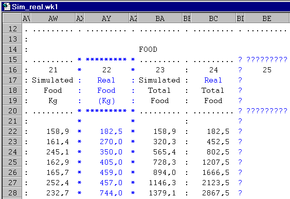
Food
This section groups the kilos of food distribution, both simulated and real.
Simulated Food kg (21) – the amount of food distributed for the week based upon DFR (19) and the Real & Simulated Number (4).
Real Food Kg (22) – the actual amount of food (in kilos) distributed during the week.
Simulated Total Food kg (23) – the sum of the Simulated Food kg (21) since the beginning of the simulation.
Real Total Food Kg (24) – the sum of the Real Food Kg (22) actually distributed since the beginning of the simulation.
User’s Choice (25) – Any additional calculation can be entered into this column.
Performance
Performance as measured economically in food and individual costs.
Simulated Food Cost (32) – the results of a look up of the Characteristics of the Alimentationusing the Simulated Mean Weight (g) (6) to obtain the granulo and the Real & Simulated Date (1) to obtain the Purchase Price (units / kilo). The Purchase Price (units / kilo) is multiplied by the Simulated Food kg (21).
Real Food Cost (33) – the multiplication of the Real Food Kg (22) distributed and Price (units / kilo).
Simulated Total Food Cost (34) – the running total of the Simulated Food Cost (32).
Real Total Food Cost (35) – the running total of the Real Food Cost (33).
Simulated Price (units/kilo) Direct Food Cost (36) – this is the original cost of the lot (Number of fish multiplied by the Price per Larvae plus the Simulated Total Food Cost (34) divided by the Simulated Biomass (Kg) (16). This give the value (in costs per kilo produced) of the cheptel, but only based upon purchase price and food costs.
Simulated Value of Individual (37) – Real & Simulated Number (4) divided by the Simulated Price (units/kilo) Direct Food Cost (36). The value added to an individual in food costs alone.
Simulated Cost per Individual in Food (38) – this is the sum of the Simulated Price (units/kilo) Direct Food Cost (36) and the Simulated Biomass (Kg) (16) divided by the Real & Simulated Number (4). The cost of every individual just in food.